Chapter 9 demonstrates several, though not all, data objects from package datasets (R version 4.5.2 (2025-10-31)) and package spatstat.data (v3.1.9).
The function calls in Chapter 9 are exclusively those provided in package base and stats (R version 4.5.2 (2025-10-31)), and in the spatstat.* family of packages.
search path & loadedNamespaces on author’s computer
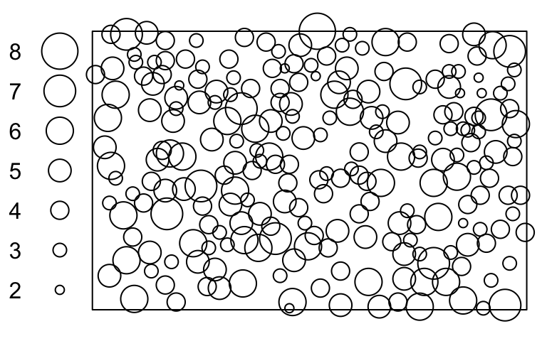
spatstat.data::anemones |> spatstat.geom::print.ppp()# Marked planar point pattern: 231 points# marks are numeric, of storage type 'integer'# window: rectangle = [0, 280] x [0, 180] units
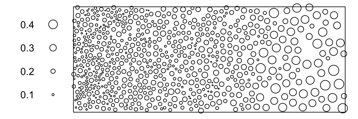
spatstat.data::bronzefilter |> spatstat.geom::print.ppp()# Marked planar point pattern: 678 points# marks are numeric, of storage type 'double'# window: rectangle = [0, 18] x [0, 7] mm
To view the hyper data frame demohyper in a desired format, readers may call the S3 method spatstat.geom::print.hyperframe() explicitly (Listing 9.27). Alternatively, readers may call the S3 generic function print() by simply typing demohyper at the R console prompt and pressing Enter, after putting the package spatstat.geom (v3.7.0.8)
either, in the search() path, by either one of the following approaches,
using the function library(), e.g., library(spatstat.geom), which is called internally by the function require();
using the function attachNamespace(), e.g., attachNamespace('spatstat.geom');
or, in the loadedNamespaces(), by either one of the following approaches,
using the function loadNamespace(), e.g., loadNamespace('spatstat.geom'), which is called internally by the function requireNamespace();
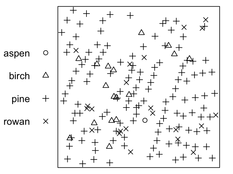
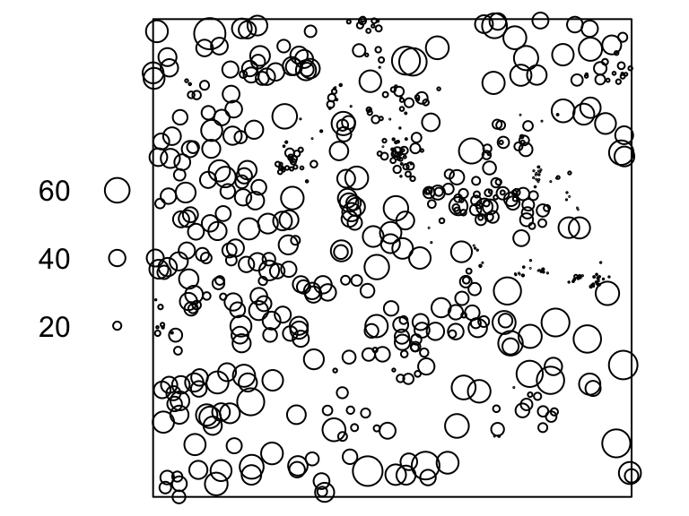
spatstat.data::longleaf |> spatstat.geom::print.ppp()# Marked planar point pattern: 584 points# marks are numeric, of storage type 'double'# window: rectangle = [0, 200] x [0, 200] metres
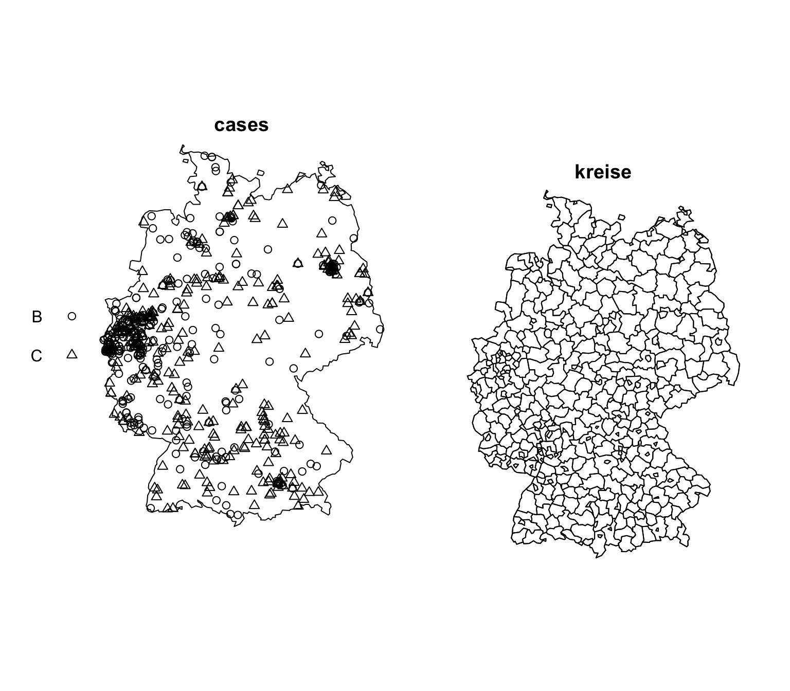
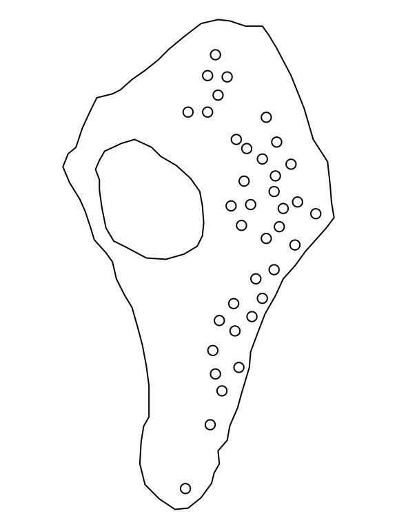
spatstat.data::meningitis# List of spatial objects# # cases:# Marked planar point pattern: 636 points# Multitype, with levels = B, C # window: polygonal boundary# enclosing rectangle: [4031.295, 4672.253] x [2684.102, 3549.931] km# # kreise:# Tessellation# Tiles are irregular polygons# 413 tiles (irregular windows)# Tessellation has a data frame of marks:# $marks: double# window: polygonal boundary# enclosing rectangle: [4031.295, 4672.253] x [2684.102, 3549.931] km
multi-type marks, e.g., $fire.type, $cause and $ign.src;
numeric marks, e.g., $fnl.size.
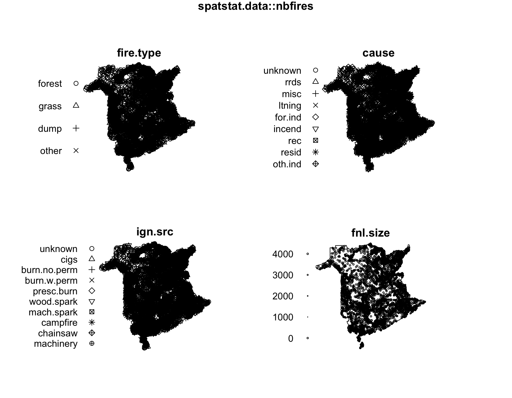
Listing 9.59: Figure: nbfires
Code
par(mar =c(0,0,1,0))spatstat.data::nbfires |> spatstat.geom::plot.ppp(which.marks =c('fire.type', 'cause', 'ign.src', 'fnl.size'))# Warning: Only 10 out of 16 symbols are shown in the symbol map
Figure 9.13: nbfires
Listing 9.60: Data: nbfires
spatstat.data::nbfires |> spatstat.geom::print.ppp()# Warning: some mark values are NA in the point pattern x# Marked planar point pattern: 7108 points# Mark variables: year, fire.type, dis.date, dis.julian, out.date, out.julian, cause, ign.src, fnl.size # window: polygonal boundary# enclosing rectangle: [0, 1000] x [0, 958.9142] units (one unit = 0.403716 km)
spatstat.data::spruces |> spatstat.geom::print.ppp()# Marked planar point pattern: 134 points# marks are numeric, of storage type 'double'# window: rectangle = [0, 56] x [0, 38] metres