library(groupedHyperframe)10 Trapezoidal Integration
The examples in Chapter 10 require
search path & loadedNamespaces on author’s computer
search()
#  [1] ".GlobalEnv"                "package:groupedHyperframe" "package:stats"             "package:graphics"          "package:grDevices"         "package:utils"             "package:datasets"
#  [8] "package:methods"           "Autoloads"                 "package:base"
loadedNamespaces() |> sort.int()
#  [1] "abind"             "base"              "cli"               "cluster"           "codetools"         "compiler"          "datasets"          "deldir"            "digest"
# [10] "doParallel"        "dplyr"             "evaluate"          "farver"            "fastmap"           "fastmatrix"        "foreach"           "generics"          "geomtextpath"
# [19] "GET"               "ggplot2"           "glue"              "goftest"           "graphics"          "grDevices"         "grid"              "gridExtra"         "groupedHyperframe"
# [28] "gtable"            "htmltools"         "htmlwidgets"       "iterators"         "jsonlite"          "knitr"             "lattice"           "lifecycle"         "magrittr"
# [37] "Matrix"            "matrixStats"       "methods"           "nlme"              "otel"              "parallel"          "patchwork"         "pillar"            "pkgconfig"
# [46] "polyclip"          "pracma"            "R6"                "RColorBrewer"      "rlang"             "rmarkdown"         "rstudioapi"        "S7"                "scales"
# [55] "SpatialPack"       "spatstat.data"     "spatstat.explore"  "spatstat.geom"     "spatstat.random"   "spatstat.sparse"   "spatstat.univar"   "spatstat.utils"    "splines"
# [64] "stats"             "survival"          "systemfonts"       "tensor"            "textshaping"       "tibble"            "tidyselect"        "tools"             "utils"
# [73] "vctrs"             "viridisLite"       "xfun"              "yaml"
10.1 Chained Trapezoidal Rule
The chained trapezoidal rule of numerically approximating a definite integral is an ancient idea since the dawn of human civilization.
Let \(\{x_k; k=0,\cdots,N\}\) be a partition of the real interval \([a,b]\) such that \(a = x_0 < x_1 < \cdots < x_{N-1} < x_N = b\) and \(\Delta x_k= x_k - x_{k-1}\) be the length of the \(k\)-th sub-interval, then the chained-trapezoidal approximation of the integration of the function \(y=f(x)\) is,
\[ \begin{split} \int_a^b f(x)\,dx & \approx \sum_{k=1}^{N}{\dfrac{y_{k-1}+y_k}{2}}\Delta x_{k} \\ & = \left(\frac{y_0}{2}+\sum _{k=1}^{N-1}y_k+\frac{y_N}{2}\right)\Delta x, \quad\iff\ \forall k, \Delta x_{k}\equiv \Delta x \end{split} \tag{10.1}\]
Listing 10.1 creates a toy example of two numeric vectors x \(=(x_0,x_1,x_2,x_3,x_4,x_5)^t\) and y \(=\{y_k = f(x_k);k=0,1,\cdots,5\}\). The numeric vector x is intentionally made non-equidistant, as neither the chained trapezoidal rule framework nor the functions pracma::trapz() and pracma::cumtrapz() (Borchers 2025, v2.4.6) requires the equidistant assumption.
x and y
x. = seq.int(from = 10L, to = 20L, by = 2L)
set.seed(23); x = rnorm(n = length(x.), mean = x., sd = .5)
set.seed(12); y = rnorm(n = length(x.), mean = 1, sd = .3)
list(x = x, y = y)
# $x
# [1] 10.09661 11.78266 14.45663 16.89669 18.49830 20.55375
#
# $y
# [1] 0.5558297 1.4731508 0.7129767 0.7239984 0.4007074 0.9183112
Listing 10.2 calculates the trapezoidal integration (Equation 10.1, Figure 10.1) of the toy example x and y (Listing 10.1).
pracma::trapz() (Listing 10.1)
pracma::trapz(x, y)
# [1] 8.642715
In R nomenclature, the term “cumulative” indicates an inclusive scan, i.e., the ith element of the output is the operation result of the first-i-elements of the input. For example, Listing 10.3 is a summation, while Listing 10.4 is a cumulative summation.
sum()
sum(1:5)
# [1] 15cumsum()
cumsum(1:5)
# [1]  1  3  6 10 15
Listing 10.5 calculates the cumulative trapezoidal integration of the toy example x and y (Listing 10.1). Note that the first element of the output is always 0, as a trapezoidal integration needs at least two points of \(\left(x_0, y_0\right)\) and \(\left(x_1, y_1\right)\).
pracma::cumtrapz() (Listing 10.1)
pracma::cumtrapz(x, y)
#          [,1]
# [1,] 0.000000
# [2,] 1.710484
# [3,] 4.633309
# [4,] 6.386462
# [5,] 7.287131
# [6,] 8.642715
10.2 (Cumulative) Average Vertical Height
The average vertical height of a trapezoidal integration is the chained-trapezoid (Equation 10.1) divided by the length of \(x\)-domain \(b-a\),
\[ \begin{split} (b-a)^{-1}\displaystyle\int_a^b f(x)\,dx & \approx (b-a)^{-1} \sum_{k=1}^{N}{\dfrac{y_{k-1}+y_k}{2}}\Delta x_{k} \\ & = N^{-1}\left(\frac{y_0}{2}+\sum _{k=1}^{N-1}y_k+\frac{y_N}{2}\right), \quad\iff\ \forall k, \Delta x_{k}\equiv \Delta x \end{split} \tag{10.2}\]
The function vtrapz() (Listing 10.6) calculates the average vertical height of a trapezoidal integration (Equation 10.2). The (tentative) prefix v indicates “vertical”. The shaded rectangle in Figure 10.1 has the same area as the trapezoidal integration. Therefore, the vertical height of the shaded rectangle is defined as the average vertical height of the trapezoidal integration.
vtrapz() (Listing 10.1)
vtrapz(x, y)
# [1] 0.8264894
The S3 generic function cumvtrapz() calculates the cumulative average vertical height of a trapezoidal integration. Package groupedHyperframe (v0.3.4) implements the following S3 methods (Table 10.1),
S3 methods of groupedHyperframe::cumvtrapz (v0.3.4)
| visible | isS4 | |
|---|---|---|
cumvtrapz.fv |
TRUE | FALSE |
cumvtrapz.fvlist |
TRUE | FALSE |
cumvtrapz.hyperframe |
TRUE | FALSE |
cumvtrapz.numeric |
TRUE | FALSE |
The S3 method cumvtrapz.numeric() takes a numeric-vector input of x. The output (Listing 10.7) has,
- the 1st element of
NaN, i.e., the result of0(trapzoidal integration) divided by0(length of \(x\)-domain). The firstNaN-value is often removed for downstream analysis using the default parameter valuerm1 = TRUE; - the 2nd element of \((y_0+y_1)/2\);
- the \((i+1)\)-th element of \(i^{-1}(y_0/2+\sum_{k=1}^{i-1}y_k+y_i/2)\), if \(\{x_k;k=0,\cdots,i\}\) are equidistant, i.e., \(\forall k\in\{1,\cdots,i\}\), \(\Delta x_{k}\equiv \Delta x\). Note that the R does not use zero-based numbering; i.e., R
vectorindices start at1Linstead of0L; - the \((N+1)\)-th and last element of Equation 10.2 (Listing 10.6).
cumvtrapz.numeric() (Listing 10.1)
cumvtrapz(x, y, rm1 = FALSE)
#           [,1]
# [1,]       NaN
# [2,] 1.0144903
# [3,] 1.0626788
# [4,] 0.9391734
# [5,] 0.8673404
# [6,] 0.8264894
10.3 Visualization
The S3 generic function visualize_vtrapz() visualizes the concept of (cumulative) average vertical height of a trapezoidal integration. Package groupedHyperframe (v0.3.4) implements the following S3 methods (Table 10.2),
S3 methods of groupedHyperframe::visualize_vtrapz (v0.3.4)
| visible | isS4 | |
|---|---|---|
visualize_vtrapz.density |
TRUE | FALSE |
visualize_vtrapz.function |
TRUE | FALSE |
visualize_vtrapz.fv |
TRUE | FALSE |
visualize_vtrapz.ksmooth |
TRUE | FALSE |
visualize_vtrapz.listof |
TRUE | FALSE |
visualize_vtrapz.loess |
TRUE | FALSE |
visualize_vtrapz.numeric |
TRUE | FALSE |
visualize_vtrapz.smooth.spline |
TRUE | FALSE |
visualize_vtrapz.spline |
TRUE | FALSE |
visualize_vtrapz.stepfun |
TRUE | FALSE |
visualize_vtrapz.xyVector |
TRUE | FALSE |
Figure 10.1 and Figure 10.2 visualize the toy example (Listing 10.1) of the non-equidistant \((x_0,x_1,\cdots,x_5)^t\) and \((y_0,y_1,\cdots,y_5)^t\), as two numeric vectors or as an 'xyVector' object (Chapter 43), respectively.
visualize_vtrapz.numeric() (Listing 10.1)
visualize_vtrapz(x, y) +
  ggplot2::theme_minimal()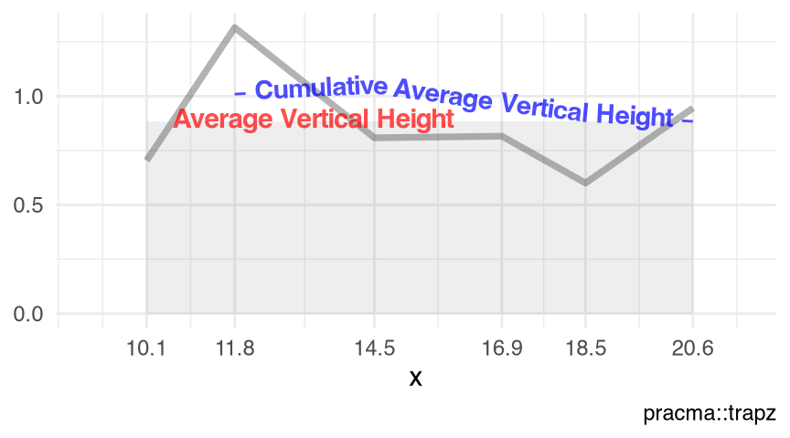
visualize_vtrapz.xyVector() (Listing 10.1)
splines::xyVector(x = x, y = y) |>
  visualize_vtrapz() +
ggplot2::theme_minimal()splines::xyVector()
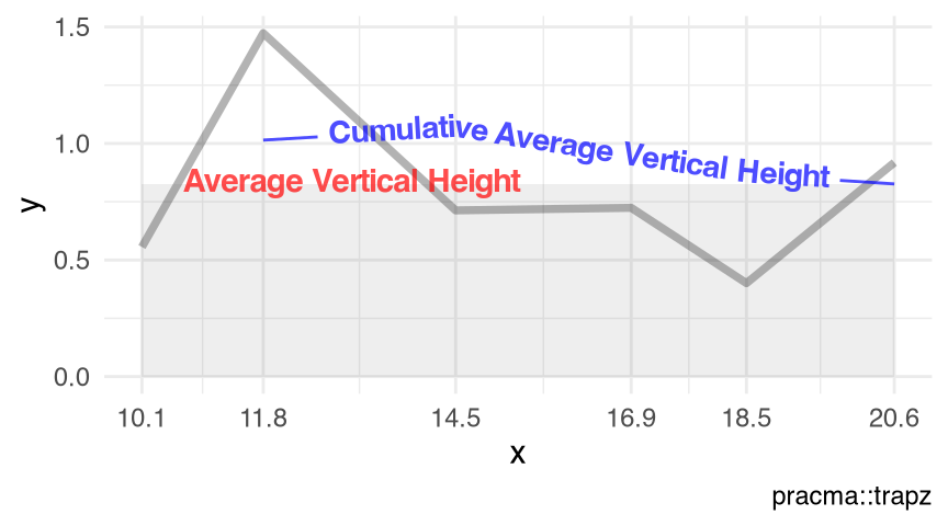
Figure 10.3 visualizes the kernel density() of a random normal sample of size 1e3L, using the elements $x and $y. Obviously, this practice is meaningless mathematically, as a density function has an \(x\)-domain of \((-\infty, \infty)\), thus the (cumulative) average vertical height of the trapzoidal integration under a density curve should be a constant of zero. This practice is meaningful to an empirical density though, if we use the range of the actual observations as the \(x\)-domain.
visualize_vtrapz.density()
set.seed(12); rnorm(n = 1e3L) |> density() |>
  visualize_vtrapz() +
ggplot2::theme_minimal()density()
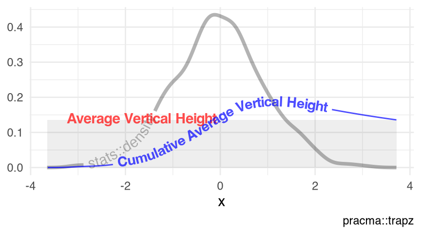
Figure 10.4 visualizes the empirical cumulative distribution function ecdf() of a random normal sample of size 1e3L, using the objects x and y in the enclosing environment. Obviously, this practice is meaningless mathematically, as a distribution function has an \(x\)-domain of \((-\infty, \infty)\), thus the (cumulative) average vertical height of the trapzoidal integration under a distribution curve should be a constant of zero. This practice is meaningful to an empirical distribution though, if we use the range of the actual observations as the \(x\)-domain.
visualize_vtrapz.stepfun()
set.seed(27); rnorm(n = 1e3L) |> ecdf() |>
  visualize_vtrapz() +
ggplot2::theme_minimal()ecdf()
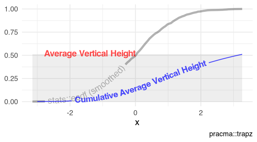
Figure 10.5 visualizes the predicted values of the local polynomial regression fit loess() with the numeric response $dist and the numeric predictor $speed in the data set cars (Section 9.7).
visualize_vtrapz.loess()
loess(dist ~ speed, data = datasets::cars) |>
  visualize_vtrapz() +
ggplot2::theme_minimal()loess()
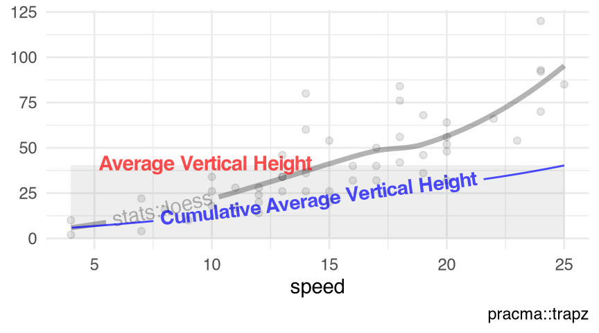
Figure 10.5 visualizes the kernel regression smoother ksmooth() with the numeric response $dist and the numeric predictor $speed in the data set cars (Section 9.7).
visualize_vtrapz.ksmooth()
datasets::cars |>
  with.default(data = _, expr = {
    ksmooth(x = speed, y = dist, kernel = 'normal', bandwidth = 2)
  }) |>
  visualize_vtrapz.ksmooth() +
  ggplot2::geom_point(
    data = datasets::cars,
    mapping = ggplot2::aes(x = speed, y = dist),
    alpha = .1
  ) +
  ggplot2::labs(x = 'speed', y = 'dist') +
ggplot2::theme_minimal()ksmooth()
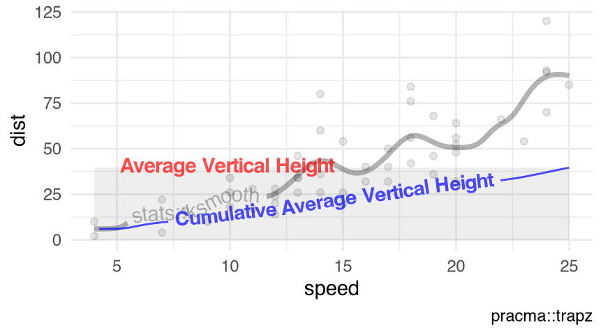
Figure 10.7 visualizes the predicted values of the smoothing spline estimates smooth.spline() with the numeric response $dist and the numeric predictor $speed in the data set cars (Section 9.7).
visualize_vtrapz.smooth.spline()
datasets::cars |>
  with.default(data = _, expr = smooth.spline(x = speed, y = dist)) |>
  visualize_vtrapz() +
ggplot2::theme_minimal()smooth.spline()
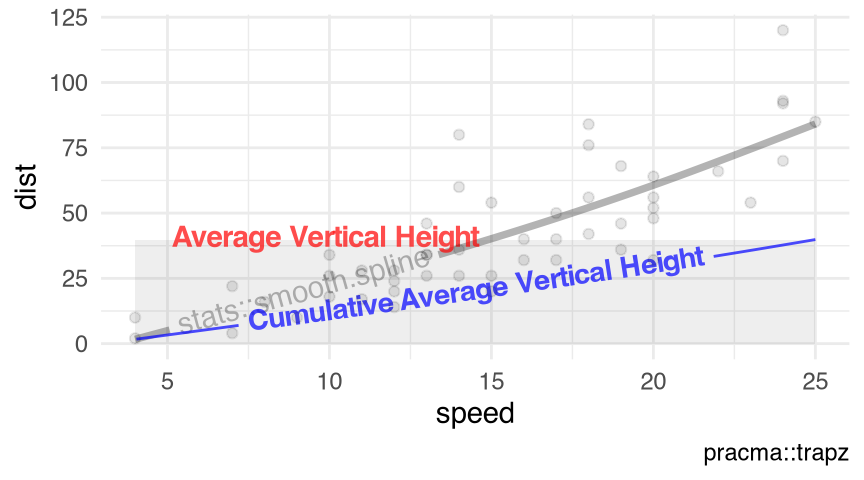
Figure 10.8 visualizes the receiver operating characteristic (ROC) curve of the point-pattern (Baddeley et al. 2025) swedishpines (Section 9.22). Note that
- the average vertical height of the trapezoidal integration under the ROC-curve of a point-pattern, via function
roc.ppp(); and - the area-under-ROC-curve (AU-ROC) of a point-pattern, via function
auc.ppp()
are mathematically equivalent, although not numerically identical (Listing 10.15, as of package spatstat.explore v3.7.0.12), because the \(x\)-domain is \([0,1]\) for an ROC curve.
roc.ppp() vs. auc.ppp()
Code
spatstat.data::swedishpines |>
  spatstat.explore::roc.ppp(covariate = 'x') |>
  spatstat.explore::with.fv(expr = {
    vtrapz(x = p, y = raw)
  }) |>
  all.equal.numeric(
    target = _,
    current = spatstat.data::swedishpines |>
      spatstat.explore::auc.ppp(covariate = 'x')
  )
# [1] "Mean relative difference: 0.0001160553"visualize_vtrapz.fv()
spatstat.data::swedishpines |>
  spatstat.explore::roc.ppp(covariate = 'x') |>
  visualize_vtrapz() +
ggplot2::theme_minimal()roc.ppp()
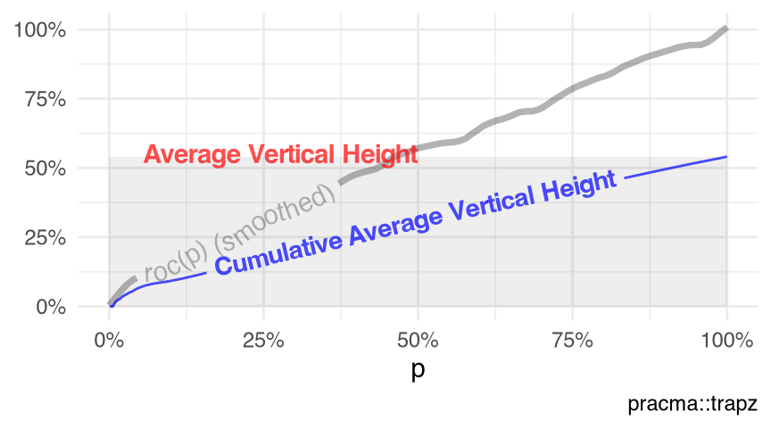
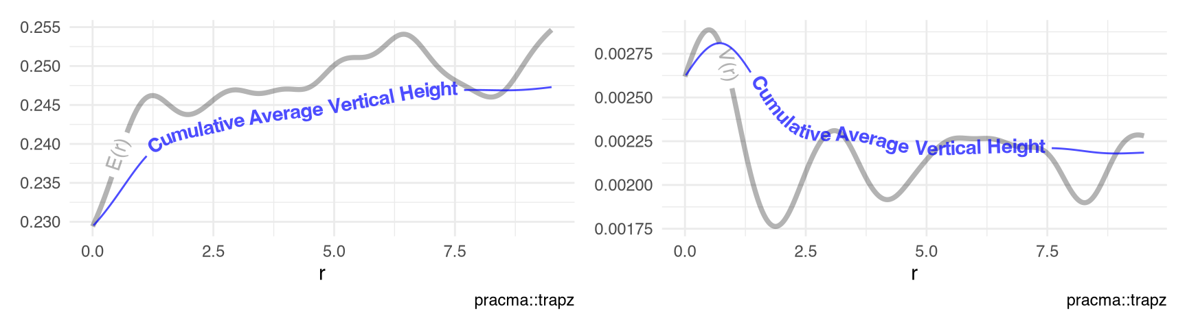
Figure 10.9 visualizes the conditional mean \(E(r)\) and variance \(V(r)\) between the points and the marks (Schlather, Ribeiro, and Diggle 2003) of the point-pattern spruces (Section 9.21) using the functions Emark() and Vmark() (v3.7.0.12).
visualize_vtrapz.listof()
list(
  spatstat.data::spruces |>
    spatstat.explore::Emark(),
  spatstat.data::spruces |>
    spatstat.explore::Vmark()
) |>
  visualize_vtrapz.listof(draw.rect = FALSE) &
ggplot2::theme_minimal()Emark() and Vmark()